One Turn After Another

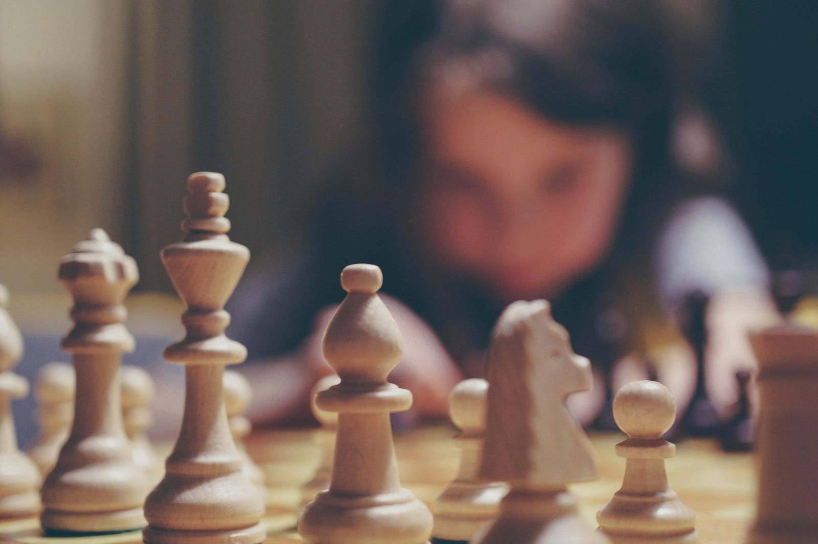
While some games, like rock-paper-scissors, only work if all payers decide on their actions simultaneously, other games, like chess or Monopoly, expect the players to take turns one after another. In Game Theory, the first kind of game is called a static game, while turn-taking is a property of so-called dynamic games. In this article, we will analyse the latter with methods from game theory. 

This article is the fourth part of a four-chapter series on the fundamentals of game theory. I recommend you to read the first three articles if you haven’t done that yet, as the concepts shown here will build on the terms and paradigms introduced in the previous articles. But if you are already familiar with the core fundamentals of game theory, don’t let yourself be stopped, and go ahead!

Dynamic games

While so far we only looked at static games, we will now introduce dynamic games where payers take turns. As previously, such games include a number of players n, a set of actions for each player, and a reward function that assesses the actions of a player given the other players’ actions. Beyond that, for a dynamic game, we need to define an order in which the players take their turns. Consider the following tree-like visualization of a dynamic game. 

At the top we have a node where player 1 has to decide between two actions L and R. This determines whether to follow the left part or the right part of the tree. After player 1’s turn, player 2 takes their turn. If player 1 chooses L, player 2 can decide between l1 and r1. If player 1 chooses R, player 2 has to decide between l2 and r2. At the leaves of the tree (the nodes at the bottom), we see the rewards just like we had them in the matrix cells in static games. For example, if player 1 decides for L and player 2 decides for r1, the reward is (1,0); that is, player 1 gets a reward of 1, and player 2 gets a reward of 0. 

I bet you are eager to find the Nash equilibrium of this game, as this is what Game Theory is mainly about (if you still struggle with the concept of Nash equilibrium, you might want to take a look back at chapter 2 of this series). To do that, we can transform the game into a matrix, as we already know how to find a Nash equilibrium in a game displayed as a matrix. Player 1 decides on the row of the matrix, player 2 decides on the column and the values in the cell then specifies the reward. However, there is one important point to notice. When we look at the game displayed as a tree, player 2 decides on their action after player 1 does and hence only cares about the part of the tree that is actually reached. If player 1 chooses action L, player 2 only decides between l1 and r1 and doesn’t care about l2 and r2, because these actions are out of the question anyway. However, when we search for a Nash Equilibrium, we need to be aware of what would happen, if player 1 would change their action. Therefore, we must know what player 2 would have done if player 1 had chosen a different option. That is why we have four columns in the following matrix, to always account for decisions in both parts of the tree. 

A column like (r1,l2) can be read as “player 2 chooses r1 if player 1 chose L and chooses l2 if player 1 chose R”. On this matrix, we can search for the best answers. For example, the cell (L, (l1,l2)) with reward 3,1 is a best answer. Player 1 has no reason to change from L to R because that would lower his reward (from 3 to 1), and Player 2 has no reason to change either because none of the other options is better (one is as good, though). In total, we find three Nash equilibria, which are underlined in the upcoming matrix: 

The chocolate-pudding market

Our next example brings the idea of dynamic games to life. Let’s assume player 2 is a market-leading retailer of chocolate pudding. Player 1 also wants to build up his business but isn’t sure yet whether to join the chocolate pudding market or whether they rather should sell something else. In our game, player 1 has the first turn and can decide between two actions. Join the market (i.e., sell chocolate pudding), or don’t join the market (i.e., sell something else). If player 1 decides to sell something other than chocolate pudding, player 2 stays the market-dominating retailer for chocolate pudding and player 1 makes some money in the other area they decided for. This is reflected by the reward 1,3 in the right part of the tree in the following figure. 

But what if player 1 is greedy for the unimaginable riches that lie dormant on the chocolate pudding market? If they decide to join the market, it is player 2’s turn. They can decide to accept the new competitor, give in and share the market. In this case, both players get a reward of 2. But player 2 can also decide to start a price war to demonstrate his superiority to the new competitor. In this case, both players get a reward of 0, because they ruin their profit due to dumping prices. 

Just like before, we can turn this tree into a matrix and find the Nash equilibria by searching for the best answers:

If player 1 joins the market, the best option for player 1 is to give in. This is an equilibrium because no player has any reason to change. For player 1 it does not make sense to leave the market (that would give a reward of 1 instead of 2) and for player 2 it is no good idea to switch to fighting either (which would give a reward of 0 instead of 2). The other Nash equilibrium happens when player 1 just doesn’t join the market. However, this scenario includes player 2’s decision to fight, if player 1 had chosen to join the market instead. He basically makes a threat and says “If you join the market, I will fight you.” Remember that previously we said we need to know what the players would do even in the cases that don’t appear to happen? Here we see why this is important. Player 1 needs to assume that player 2 would fight because that is the only reason for player 1 to stay out of the market. If player 2 wouldn’t threaten to fight, we wouldn’t have a Nash equilibrium, because then joining the market would become a better option for player 1. 

But how reasonable is this threat? It keeps player 1 outside the market, but what would happen if player 1 didn’t believe the threat and decided to still join the market? Would player 2 really carry out his threat and fight? That would be very silly because it would give him a reward of 0, whereas giving in would give a reward of 2. From that perspective, player 2 used an empty threat that is not very reasonable. If the case really occurs, he wouldn’t carry it out anyway, would he?

Subgame perfect equilibrium

The previous example showed that sometimes Nash equilibria occur, that are not very reasonable within the game. To cope with this problem, a more strict concept of equilibrium has been introduced which is called a subgame perfect equilibrium. This adds some stricter conditions to the notion of an equilibrium. Hence every subgame perfect equilibrium is a Nash equilibrium, but not all Nash equilibria are subgame perfect. 

A Nash equilibrium is subgame perfect if every subgame of this equilibrium is a Nash equilibrium itself. What does that mean? First, we have to understand that a subgame is a part of the game’s tree that starts at any node. For example, if player 1 chooses L, the remainder of the tree under the node reached by playing L is a subgame. In a likewise fashion, the tree that comes after the node of action R is a subgame. Last but not least, the whole game is always a subgame of itself. As a consequence, the example we started with has three subgames, which are marked in grey, orange and blue in the following: 

We already saw, that this game has three Nash equilibria which are (L,(l1,l2)), (L, (l1,r2)) and (R,(r1,r2)). Let us now find out which of these are subgame perfect. To this end, we investigate the subgames one after another, starting with the orange one. If we only look at the orange part of the tree, there is a single Nash equilibrium that occurs if player 2 chooses l1. If we look at the blue subgame, there is also a single Nash equilibrium that is reached when player 2 chooses r2. Now that tells us that in every subgame perfect Nash equilibrium, player 2 has to choose option l1 if we arrive in the orange subgame (i.e. if player 1 chooses L) and player 2 has to choose option r2 if we arrive at the blue subgame (i.e., if player 1 chooses R). Only one of the previous Nash equilibria fulfills this condition, namely (L,(l1,r2)). Hence this is the only subgame perfect Nash equilibrium of the whole game. The other two versions are Nash equilibria as well, but they are somewhat unlogical in the sense, that they contain some kind of empty threat, as we had it in the chocolate pudding market example before. The method we just used to find the subgame perfect Nash equilibrium is called backwards induction, by the way. 

Uncertainty

So far in our dynamic games, we always knew which decisions the other players made. For a game like chess, this is the case indeed, as every move your opponent makes is perfectly observable. However, there are other situations in which you might not be sure about the exact moves the other players make. As an example, we go back to the chocolate pudding market. You take the perspective of the retailer that is already in the market and you have to decide whether you would start fighting if the other player joins the market. But there is one thing you don’t know, namely how aggressive your opponent will be. When you start fighting, will they be frightened easily and give up? Or will they be aggressive and fight you until only one of you is left? This can be seen as a decision made by the other player that influences your decision. If you expect the other player to be a coward, you might prefer to fight, but if they turn out to be aggressive, you would rather want to give in (reminds you of the birds fighting for food in the previous chapter, doesn’t it?). We can model this scenario in a game like this: 

The dotted circle around the two nodes indicates, that these are hidden decisions that are not observable to everyone. If you are player 2, you know whether player 1 joined the market or not, but if they joined, you don’t know whether they are aggressive (left node) or moderate (right node). Hence you act under uncertainty, which is a very common ingredient in many games you play in the real world. Poker would become very boring if everybody knew everyone’s cards, that’s why there is private information, namely the cards on your hand only you know about. 

Now you still have to decide whether to fight or give in, although you are not exactly sure what node of the tree you are in. To do that, you have to make assumptions about the likelihood of each state. If you are quite certain that the other player is behaving moderately, you might be up for a fight, but if you assume them to be aggressive, you might prefer giving in. Say there is a Probability p that the other player is aggressive and 1-p that they behave moderately. If you assume p to be high, you should give in, but if p becomes smaller, there should be a point where your decision switches to fighting. Let’s try to find that point. In particular, there should be a sweet spot in between where the probability of the other player being aggressive vs. moderate is such that fighting and giving in are equal alternatives to one another. That is, the rewards would be equal, which we can model as follows: 

Do you see how this formula is derived from the rewards for fighting or giving in in the different leaves of the tree? This formula solves to p=1/3, so if the probability of the other player being aggressive is 1/3 it would make no difference whether to fight or give in. But if you assume the other player to be aggressive with a probability of more than 1/3, you should give in, and if you assume aggressiveness to be less likely than 1/3, you should fight. This is a chain of thought you also have in other games where you act under uncertainty. When you play poker, you might not calculate the probabilities exactly, but you ask yourself, “How likely is it that John has two kings on his hand?” and depending on your assumption of that probability, you check, raise or give up. 

Summary & outlook

Now we have learned a lot about dynamic games. Let us summarize our key findings. 

• Dynamic games include an order in which players take turns. 
• In dynamic games, the players’ possible actions depend on the previously executed actions of the other players. 
• A Nash equilibrium in a dynamic game can be implausible, as it contains an empty threat that would not be rational.
• The concept of subgame perfect equilibria prevents such implausible solutions. 
• In dynamic games, decisions can be hidden. In that case, players may not exactly know which node of the game they are in and have to assign probabilities to different states of the games. 

With that, we have reached the end of our series on the fundamentals of game theory. We have learned a lot, yet there are plenty of things we haven’t been able to cover. Game theory is a science in itself, and we have only been able to scratch the surface. Other concepts that expand the possibilities of game-theoretic analyses include: 

• Analysing games that are repeated multiple times. If you play the prisoner’s dilemma multiple times, you might be tempted to punish the other player for having betrayed you in the previous round. 
• In cooperative games, players can conclude binding contracts that determine their actions to reach a solution of the game together. This is different from the non-cooperative games we looked at, where all players are free to decide and maximize their own reward. 
• While we only looked at discrete games, where each player has a finite number of actions to choose from, continuous games allow an infinite number of actions (e.g., any number between 0 and 1). 
• A big part of game theory considers the usage of public goods and the problem that individuals might consume these goods without contributing to their maintenance. 

These concepts allow us to analyse real-world scenarios from various fields such as auctions, social networks, evolution, markets, information sharing, voting behaviour and much more. I hope you enjoyed this series and find meaningful applications for the knowledge you gained, be it the analysis of customer behaviour, political negotiations or the next game night with your friends. From a game theory perspective, life is a game!

References

The topics introduced here are typically covered in standard textbooks on game theory. I mainly used this one, which is written in German though:

• Bartholomae, F., & Wiens, M. (2016). Spieltheorie. Ein anwendungsorientiertes Lehrbuch. Wiesbaden: Springer Fachmedien Wiesbaden.

An alternative in the English language could be this one:

• Espinola-Arredondo, A., & Muñoz-Garcia, F. (2023). Game Theory: An Introduction with Step-by-step Examples. Springer Nature.

Game theory is a rather young field of research, with the first main textbook being this one:

• Von Neumann, J., & Morgenstern, O. (1944). Theory of games and economic behavior.

Like this article? Follow me to be notified of my future posts.

The post One Turn After Another appeared first on Towards Data Science.