MongoDB with Search Indexes Queried as Kimball's Star Schema with Facts and Dimensions

Export From SQL to CSV Import to MongoDB Indexing the Star Schema Querying the Star Schema - Star Transformation MongoDB queries on a Star Schema Conclusion In document databases like MongoDB, data modeling is typically optimized for predefined access patterns, where each domain or service owns its database. This contrasts with the relational model, which often serves as a centralized, fully normalized database designed independently of any specific application. However, most applications also require the ability to perform ad-hoc queries or real-time analytics, where the query patterns are not predetermined. Here, it is the opposite: SQL requires another database schema, whereas MongoDB offers the same dimensional model approach on the operational database. In relational databases, a common practice is to create a separate analytics database, often in a dimensional model like the star schema popularized by Ralph Kimball. Here, normalized fact tables are surrounded by denormalized dimension tables. This setup is separate from the operational database and not updated in real-time by transactional workloads. MongoDB, allows for a different strategy. Thanks to features like MongoDB Atlas Search Indexes, real-time analytics can be performed directly on the operational database without the need for replication to a separate analytical database. Here is a simple example using the Oracle Sales History Sample Schema which I used a lot in the past as an example of a Star Schema designed correctly with Bitmap Indexes on Foreign Keys to allow Star transformation. Export From SQL to CSV The simplest to get the Sales History Sample Schema (SH) populated with data is having an Autonomous Database on the Oracle Cloud Free Tier, as it is created by default. I used SQLcl UNLOAD to get data into CSV files: for i in CHANNELS COSTS COUNTRIES CUSTOMERS PRODUCTS PROMOTIONS SALES SUPPLEMENTARY_DEMOGRAPHICS TIMES do echo "set loadformat csv" echo "alter session set nls_date_format = 'YYYY-MM-DD';" echo "unload SH.$i" done > unload.sql sqlcl @ unload.sql This generated the following CSV files, in the current directory: $ wc -l *.csv | sort -n 6 CHANNELS_DATA_TABLE.csv 24 COUNTRIES_DATA_TABLE.csv 73 PRODUCTS_DATA_TABLE.csv 504 PROMOTIONS_DATA_TABLE.csv 1827 TIMES_DATA_TABLE.csv 4501 SUPPLEMENTARY_DEMOGRAPHICS_DATA_TABLE.csv 55501 CUSTOMERS_DATA_TABLE.csv 82113 COSTS_DATA_TABLE.csv 918844 SALES_DATA_TABLE.csv The CSV files contain a header with the column names used in the star schema: Image from: https://docs.oracle.com/cd/B19306_01/server.102/b14198/graphics/comsc007.gif Import to MongoDB I started a local MongoDB Atlas: atlas deployments setup atlas --type local --port 27017 --force I imported the CSV files: mongoimport -j 8 --type=csv --headerline --drop --file=CHANNELS_DATA_TABLE.csv --db=sh --collection=channels $@ && mongoimport -j 8 --type=csv --headerline --drop --file=COSTS_DATA_TABLE.csv --db=sh --collection=costs && mongoimport -j 8 --type=csv --headerline --drop --file=COUNTRIES_DATA_TABLE.csv --db=sh --collection=countries && mongoimport -j 8 --type=csv --headerline --drop --file=CUSTOMERS_DATA_TABLE.csv --db=sh --collection=customers && mongoimport -j 8 --type=csv --headerline --drop --file=PRODUCTS_DATA_TABLE.csv --db=sh --collection=products && mongoimport -j 8 --type=csv --headerline --drop --file=PROMOTIONS_DATA_TABLE.csv --db=sh --collection=promotions && mongoimport -j 8 --type=csv --headerline --drop --file=SALES_DATA_TABLE.csv --db=sh --collection=sales && mongosh sh --eval "show collections" It imports nine hundred thousand facts and the related dimensions in ten seconds: I connect to the "sh" database and list an example of the "sales" documents: mongosh use sh; db.sales.find().limit(2) Indexing the Star Schema In SQL databases, a single optimal index cannot be created for a Data Mart queried on multiple dimension combinations. The SH schema in Oracle Database utilizes one bitmap index for each foreign key in the fact table. Queries read all necessary indexes and combine results with bitmap operations, which is ideal when individual predicates lack selectivity, but their combinations reduce it to a small set of rows to read from the fact table. Bitmap indexes are effective for data warehouses but not for operational databases, as

Apr 13, 2025 - 22:12

MongoDB with Search Indexes Queried as Kimball's Star Schema with Facts and Dimensions

Export From SQL to CSV
Import to MongoDB
Indexing the Star Schema
Querying the Star Schema - Star Transformation
MongoDB queries on a Star Schema
Conclusion

In document databases like MongoDB, data modeling is typically optimized for predefined access patterns, where each domain or service owns its database. This contrasts with the relational model, which often serves as a centralized, fully normalized database designed independently of any specific application.
However, most applications also require the ability to perform ad-hoc queries or real-time analytics, where the query patterns are not predetermined.
Here, it is the opposite: SQL requires another database schema, whereas MongoDB offers the same dimensional model approach on the operational database.

In relational databases, a common practice is to create a separate analytics database, often in a dimensional model like the star schema popularized by Ralph Kimball. Here, normalized fact tables are surrounded by denormalized dimension tables. This setup is separate from the operational database and not updated in real-time by transactional workloads.

MongoDB, allows for a different strategy. Thanks to features like MongoDB Atlas Search Indexes, real-time analytics can be performed directly on the operational database without the need for replication to a separate analytical database. Here is a simple example using the Oracle Sales History Sample Schema which I used a lot in the past as an example of a Star Schema designed correctly with Bitmap Indexes on Foreign Keys to allow Star transformation.

Export From SQL to CSV

The simplest to get the Sales History Sample Schema (SH) populated with data is having an Autonomous Database on the Oracle Cloud Free Tier, as it is created by default.

I used SQLcl UNLOAD to get data into CSV files:

for i in CHANNELS COSTS COUNTRIES CUSTOMERS PRODUCTS PROMOTIONS SALES SUPPLEMENTARY_DEMOGRAPHICS TIMES 
do 
 echo "set loadformat csv"
 echo "alter session set nls_date_format = 'YYYY-MM-DD';"
 echo "unload SH.$i"
done > unload.sql

sqlcl @ unload.sql

This generated the following CSV files, in the current directory:


$ wc -l *.csv | sort -n                                                                                                                                                              
       6 CHANNELS_DATA_TABLE.csv
      24 COUNTRIES_DATA_TABLE.csv
      73 PRODUCTS_DATA_TABLE.csv
     504 PROMOTIONS_DATA_TABLE.csv
    1827 TIMES_DATA_TABLE.csv
    4501 SUPPLEMENTARY_DEMOGRAPHICS_DATA_TABLE.csv
   55501 CUSTOMERS_DATA_TABLE.csv
   82113 COSTS_DATA_TABLE.csv
  918844 SALES_DATA_TABLE.csv

The CSV files contain a header with the column names used in the star schema:

Image from: https://docs.oracle.com/cd/B19306_01/server.102/b14198/graphics/comsc007.gif

Import to MongoDB

I started a local MongoDB Atlas:

atlas deployments setup  atlas --type local --port 27017 --force

I imported the CSV files:

mongoimport -j 8 --type=csv --headerline --drop --file=CHANNELS_DATA_TABLE.csv --db=sh --collection=channels $@ &&                                                               
mongoimport -j 8 --type=csv --headerline --drop --file=COSTS_DATA_TABLE.csv --db=sh --collection=costs &&                                                                     
mongoimport -j 8 --type=csv --headerline --drop --file=COUNTRIES_DATA_TABLE.csv --db=sh --collection=countries &&                                                             
mongoimport -j 8 --type=csv --headerline --drop --file=CUSTOMERS_DATA_TABLE.csv --db=sh --collection=customers &&                                                             
mongoimport -j 8 --type=csv --headerline --drop --file=PRODUCTS_DATA_TABLE.csv --db=sh --collection=products &&                                                               
mongoimport -j 8 --type=csv --headerline --drop --file=PROMOTIONS_DATA_TABLE.csv --db=sh --collection=promotions &&                                                           
mongoimport -j 8 --type=csv --headerline --drop --file=SALES_DATA_TABLE.csv --db=sh --collection=sales &&
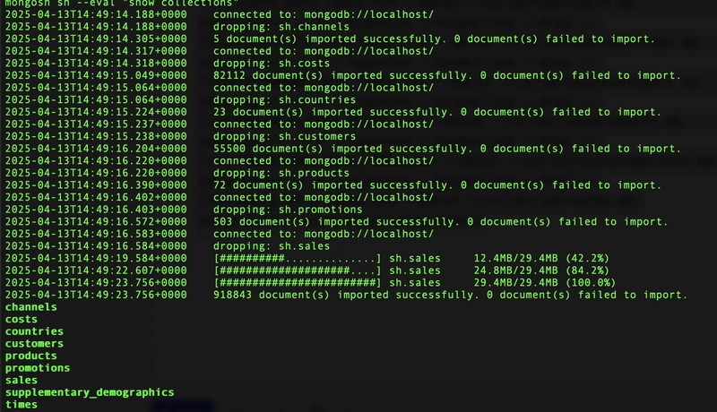
mongosh sh --eval "show collections"

It imports nine hundred thousand facts and the related dimensions in ten seconds:

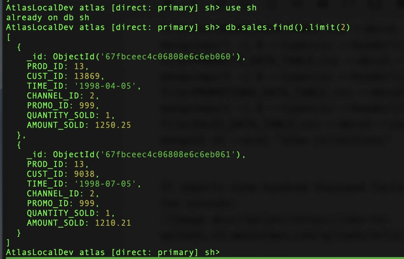
I connect to the "sh" database and list an example of the "sales" documents:

mongosh
use sh;
db.sales.find().limit(2)

Indexing the Star Schema

In SQL databases, a single optimal index cannot be created for a Data Mart queried on multiple dimension combinations. The SH schema in Oracle Database utilizes one bitmap index for each foreign key in the fact table.
Queries read all necessary indexes and combine results with bitmap operations, which is ideal when individual predicates lack selectivity, but their combinations reduce it to a small set of rows to read from the fact table.
Bitmap indexes are effective for data warehouses but not for operational databases, as they can lead to index fragmentation and locking issues in OLTP systems. For real-time analytics, Oracle offers an In-Memory Column Store, which serves as an analytic-optimized cache for transactional databases.

MongoDB has a different solution: it can serve ad-hoc queries from a single Search Index per fact table. Atlas Search indexes run within the operational database and are asynchronously updated from the change stream, allowing near real-time analytics on operational databases.

I declared the following Search Index on the dimension key fields in the fact table:

db.sales.createSearchIndex(
   "SalesDimension",
   {
     "mappings": {
       "fields": {
         "PROD_ID":    { "type": "number" },
         "CUST_ID":    { "type": "number" },
         "TIME_ID":    { "type": "token" },
         "CHANNEL_ID": { "type": "number" },
         "PROMO_ID":   { "type": "number" },
       }
     }
   }
)

I imported data directly from the CSV without defining datatypes. The TIME_ID is a character string in the YYYY-MM-DD format, so I declared it as a token. The other fields are numbers. All fields serve as foreign keys referencing dimension collections. Their values are less important than having a natural order, which may facilitate range queries.

This example can be run on MongoDB Atlas free tier (M0) which allows three Search Indexes:

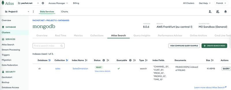
The total size of the SH schema, without the search index, is 60MB:

Logical Data Size: 172.12 MB
Storage Size: 31.49 MB
Index Size: 30.32 MB
Total Collections: 9

which is mostly the sales collection:

Storage Size: 20.83MB
Logical Data Size: 124.4MB
Total Documents: 918843
Indexes Total Size: 26.01MB

The Search Index takes approximately the same size:

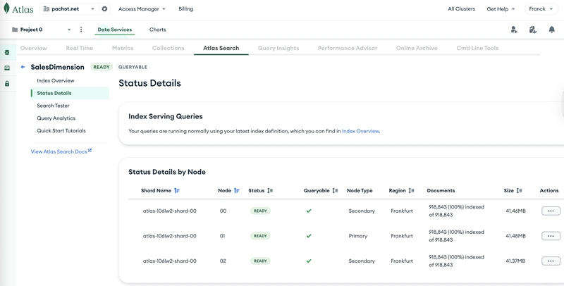
This demo showcases a small database, illustrating the value of this approach when applied to larger databases. It is recommended to compare the size of the search index with the instance memory.

Querying the Star Schema - Star Transformation

The star schema's primary advantage lies in its fact table, which contains numerous rows with limited size, holding only dimension foreign keys and measures. This large row count is offset by the smaller row size. Ideally, there is one fact table to minimize joins across many rows.
Dimension tables are smaller yet can accommodate larger rows with multiple attributes for user-defined filtering and displaying long descriptions. In SQL, queries join the fact table to dimensions in the FROM clause, while predicates are specified in the WHERE clause. The RDBMS optimizer may transform the query to leverage the star schema efficiently, as I detailed in an old article for the SOUG newsletter:

Star Transformation, 12c Adaptive Bitmap Pruning and In-Memory option | PDF

Star Transformation, 12c Adaptive Bitmap Pruning and In-Memory option - Download as a PDF or view online for free

slideshare.net

The WHERE clause predicates are applied to small dimensions to obtain the list of dimension keys. This list is then used to access the fact table through bitmap indexes, retrieving only the necessary rows. Finally, this result is joined back with dimension tables for additional projections. This transformation, available in commercial RDBMS like Oracle Database Enterprise Edition, optimizes filtering to minimize unnecessary joins. It is not available in Oracle Standard Edition or PostgreSQL.

Whether this transformation is implemented or not, an SQL query uses joins between the fact table and dimensions. For example the following query retreives the sales sales transactions from 2001 that are associated with high-cost promotions, involve customers from California, and occur through the Direct Sales channel, specifically focusing on Saturdays:

SELECT
  s.PROMO_ID, s.CUST_ID, s.CHANNEL_ID, s.TIME_ID, s.PROD_ID,
  p.PROD_NAME, p.PROD_LIST_PRICE,
  s.quantity_sold, s.amount_sold,
FROM  sales s
 JOIN products p ON s.PROD_ID = p.PROD_ID
 JOIN promotions pr ON s.PROMO_ID = pr.PROMO_ID
 JOIN customers c ON s.CUST_ID = c.CUST_ID
 JOIN channels ch ON s.CHANNEL_ID = ch.CHANNEL_ID
 JOIN times t ON s.TIME_ID = t.TIME_ID
WHERE pr.PROMO_COST > 10000
  AND c.CUST_STATE_PROVINCE = 'CA'
  AND ch.CHANNEL_DESC = 'Direct Sales'
  AND t.FISCAL_YEAR = 2001
  AND t.DAY_NAME = 'Saturday'
  AND s.TIME_ID > date '2001-01-01'
;

SQL operates independently of the physical data model. The query planner must estimate the optimal order for joining tables and selecting indexes, relying on complex combinations of predicates to assess cardinalities.

MongoDB queries on a Star Schema

MongoDB gives more control to the developer on how data is accessed, and the same optimal approach can be used:

get an array of references from each dimension where the filters are applied
query the fact table with an aggregation pipeline using the search index to find those references
lookup to the dimensions from which more fields are needed

The bitmap step is unnecessary because the search indexes, which are based on Apache Lucene, can effectively combine multiple filters with the compound operator. The dimension keys gathered as an array is simple to use with the in operator.

Here is an example to retrieve sales transactions from 2001 (TIME_ID: { $gt: "2001-01-01" }) that are associated with high-cost promotions (PROMO_COST: { $gt: 10000 }), involve customers from California ({ CUST_STATE_PROVINCE: 'CA' }), and occur through the Direct Sales channel ({ CHANNEL_DESC: 'Direct Sales' }), specifically focusing on Saturdays ({ FISCAL_YEAR: 2001 , DAY_NAME: 'Saturday' }).

For the time range, as the dimension key holds all information with its YYYY-MM-DD format, I don't need to read from the dimension. For the others, I query the dimension collections to get an array of keys that verify my condition:

const promoIds = db.promotions.find( 
 {PROMO_COST: { $gt: 10000 }} 
).toArray().map(doc => doc.PROMO_ID);

const custIds  = db.customers.find( 
  { CUST_STATE_PROVINCE: 'CA' }      
).toArray().map(doc => doc.CUST_ID);

const channelIds  = db.channels.find( 
  { CHANNEL_DESC: 'Direct Sales' } 
).toArray().map(doc => doc.CHANNEL_ID);

const timeIds  = db.times.find( 
 { FISCAL_YEAR: 2001 , DAY_NAME: 'Saturday' } 
).toArray().map(doc => doc.TIME_ID);

Don't worry about long lists, the search indexes can handle that:

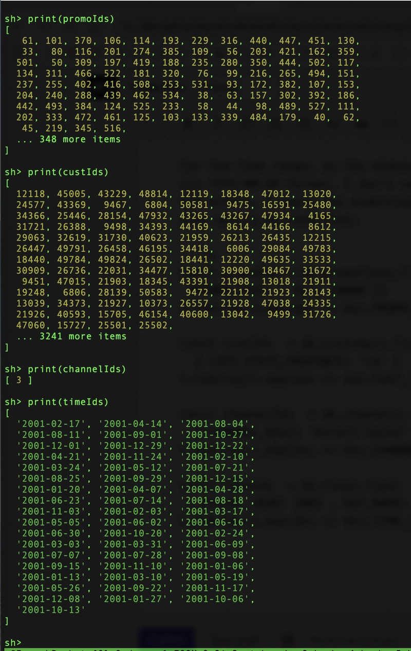
The next step is an aggregation pipeline that uses those lists, and add the time range, in a compound filter:

db.sales.aggregate([
  {
    "$search": {
      "index": "SalesDimension",
      "compound": {
        "must": [
          { "in": { "path": "PROMO_ID". , "value": promoIds   } },
          { "in": { "path": "CUST_ID".  , "value": custIds    } },
          { "in": { "path": "CHANNEL_ID", "value": channelIds } },
          { "in": { "path": "TIME_ID".  , "value": timeIds    } },
          { "range": { "path": "TIME_ID", "gt": "2001-01-01"  } }
        ]
      }
    }
  },
  { "$sort": { "TIME_ID": -1 } },
  { "$limit": 3 },
  {
    "$lookup": {
      "from":         "products",
      "localField":   "PROD_ID",
      "foreignField": "PROD_ID",
      "as":           "product_info"
    }
  },
  {
    "$unwind": "$product_info"
  },
  {
    "$project": {
      "PROMO_ID": 1,
      "CUST_ID": 1,
      "CHANNEL_ID": 1,
      "TIME_ID": 1,
      "PROD_ID": 1,
      "quantity_sold": 1,
      "amount_sold": 1,
      "product_info.PROD_NAME": 1,
      "product_info.PROD_LIST_PRICE": 1
    }
  }
]);

The search operation is the first step of the aggregation pipeline, to get efficiently the minimal items requried by the query, and further processing can be added.
I've added a sort and limit operation here to display only the last three sales. I've added more information with a lookup on the product dimension, and unwind to project only the name and price.

The result is a collection of documents ready to return to the user, returned in 8 milliseconds:

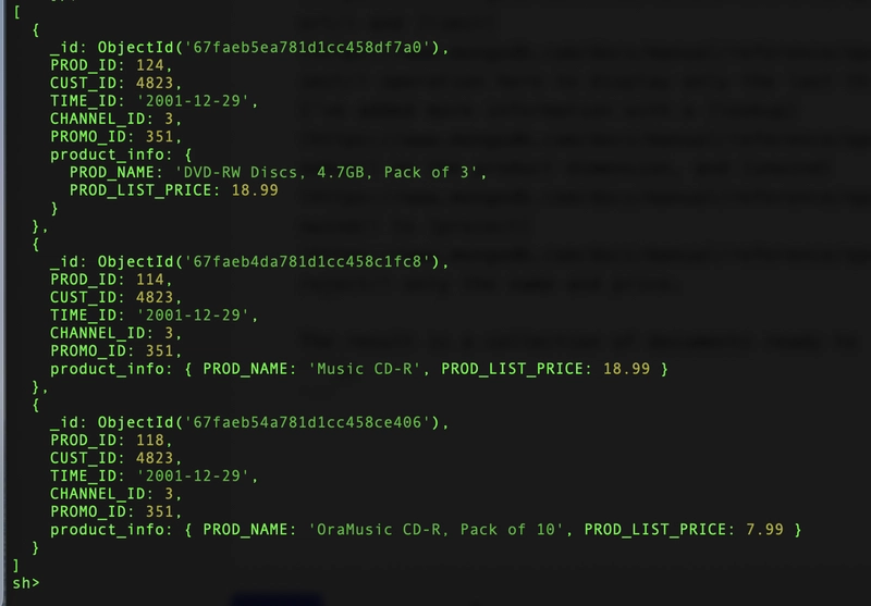
This post aims to demonstrate the search component of the analytic query by reading only the necessary documents from the fact collection. Further analytics can be appended to the aggregation pipeline. The datamodel can be improved (using better datatypes, keys as _id, and index clustering) but the goal was to show how we can run efficent analytic queries without changing the schema.

Conclusion

Unlike SQL star schemas, which necessitate Extract-Load-Transform (ELT) processes to another database, MongoDB’s document model allows transactions, including embedded or referenced data, to be stored in a single collection, effectively addressing multi-granularity facts without complex joins.

The Star Transformation approach can be used to generate a list of keys from lookup collections with applicable filters, similar to dimension tables. Atlas Search indexes combine these keys to retrieve necessary documents from the facts collection for further analysis in the aggregation pipeline.

With MongoDB, if you modeled your data properly for domain use cases and later encounter new query requirements needing scattered document aggregation, consider whether a search index can address these needs before changing the model or streaming to another database.