


![Apple Shares Official Teaser for 'Highest 2 Lowest' Starring Denzel Washington [Video]](https://www.iclarified.com/images/news/97221/97221/97221-640.jpg)

![New Powerbeats Pro 2 Wireless Earbuds On Sale for $199.95 [Lowest Price Ever]](https://www.iclarified.com/images/news/97217/97217/97217-640.jpg)
![Under-Display Face ID Coming to iPhone 18 Pro and Pro Max [Rumor]](https://www.iclarified.com/images/news/97215/97215/97215-640.jpg)


![[The AI Show Episode 145]: OpenAI Releases o3 and o4-mini, AI Is Causing “Quiet Layoffs,” Executive Order on Youth AI Education & GPT-4o’s Controversial Update](https://www.marketingaiinstitute.com/hubfs/ep%20145%20cover.png)


Diffusion Models, Explained Simply
From noise to art: how to generate high-quality images using diffusion models The post Diffusion Models, Explained Simply appeared first on Towards Data Science.

Introduction
Generative AI is one of the most popular terms we hear today. Recently, there has been a surge in generative AI applications involving text, image, audio, and video generation.
When it comes to image creation, Diffusion models have emerged as a state-of-the-art technique for content generation. Although they were first introduced in 2015, they have seen significant advancements and now serve as the core mechanism in well-known models such as DALLE, Midjourney, and CLIP.
The goal of this article is to introduce the core idea behind diffusion models. This foundational understanding will help in grasping more advanced concepts used in complex diffusion variants and in interpreting the role of hyperparameters when training a custom diffusion model.
Diffusion
Analogy from physics
Let us imagine a transparent glass of water. What happens if we add a small amount of another liquid with a yellow color, for example? The yellow liquid will gradually and uniformly spread throughout the glass, and the resulting mixture will take on a slightly transparent yellow tint.

The described process is known as forward diffusion: we altered the environment’s state by adding a small amount of another liquid. However, would it be just as easy to perform reverse diffusion — to return the mixture back to its original state? It turns out that it is not. In the best-case scenario, achieving this would require highly sophisticated mechanisms.
Applying the analogy to machine learning
Diffusion can also be applied to images. Imagine a high-quality photo of a dog. We can easily transform this image by gradually adding random noise. As a result, the pixel values will change, making the dog in the image less visible or even unrecognizable. This transformation process is known as forward diffusion.

We can also consider the inverse operation: given a noisy image, the goal is to reconstruct the original image. This task is much more challenging because there are far fewer highly recognizable image states compared to the vast number of possible noisy variations. Using the same physics analogy mentioned earlier, this process is called reverse diffusion.
Architecture of diffusion models
To better understand the structure of diffusion models, let us examine both diffusion processes separately.
Forward diffusion
As mentioned earlier, forward diffusion involves progressively adding noise to an image. In practice, however, the process is a bit more nuanced.
The most common method involves sampling a random value for each pixel from a Gaussian distribution with a mean of 0. This sampled value — which can be either positive or negative — is then added to the pixel’s original value. Repeating this operation across all pixels results in a noisy version of the original image.

The chosen Gaussian distribution typically has a relatively small variance, meaning that the sampled values are usually small. As a result, only minor changes are introduced to the image at each step.
Forward diffusion is an iterative process in which noise is applied to the image multiple times. With each iteration, the resulting image becomes increasingly dissimilar to the original. After hundreds of iterations — which is common in real diffusion models — the image eventually becomes unrecognizable from pure noise.
Reverse diffusion
Now you might ask: what is the purpose of performing all these forward diffusion transformations? The answer is that the images generated at each iteration are used to train a neural network.
Specifically, suppose we applied 100 sequential noise transformations during forward diffusion. We can then take the image at each step and train the neural network to reconstruct the image from the previous step. The difference between the predicted and actual images is calculated using a loss function — for example, Mean Squared Error (MSE), which measures the average pixel-wise difference between the two images.

This example shows a diffusion model reconstructing the original image. At the same time, diffusion models can be trained to predict the noise added to an image. In that case, to reconstruct the original image, it is sufficient to subtract the predicted noise from the image at the previous iteration.
While both of these tasks might seem similar, predicting the added noise is simpler compared to image reconstruction.
Model design
After gaining a basic intuition about the diffusion technique, it is essential to explore several more advanced concepts to better understand diffusion model design.
Number of iterations
The number of iterations is one of the key parameters in diffusion models:
On one hand, using more iterations means that image pairs at adjacent steps will differ less, making the model’s learning task easier. On the other hand, a higher number of iterations increases computational cost.
While fewer iterations can speed up training, the model may fail to learn smooth transitions between steps, resulting in poor performance.
Typically, the number of iterations is chosen between 50 and 1000.
Neural network architecture
Most commonly, the U-Net architecture is used as the backbone in diffusion models. Here are some of the reasons why:
- U-Net preserves the input and output image dimensions, ensuring that the image size remains consistent throughout the reverse diffusion process.
- Its bottleneck architecture enables the reconstruction of the entire image after compression into a latent space. Meanwhile, key image features are retained through skip connections.
- Originally designed for biomedical image segmentation, where pixel-level accuracy is crucial, U-Net’s strengths translate well to diffusion tasks that require precise prediction of individual pixel values.

Shared network
At first glance, it might seem necessary to train a separate neural network for each iteration in the diffusion process. While this approach is feasible and can lead to high-quality inference results, it is highly inefficient from a computational perspective. For example, if the diffusion process consists of a thousand steps, we would need to train a thousand U-Net models — an extremely time-consuming and resource-intensive task.
However, we can observe that the task configuration across different iterations is essentially the same: in each case, we need to reconstruct an image of identical dimensions that has been altered with noise of a similar magnitude. This important insight leads to the idea of using a single, shared neural network across all iterations.
In practice, this means that we use a single U-Net model with shared weights, trained on image pairs from different diffusion steps. During inference, the noisy image is passed through the same trained U-Net multiple times, gradually refining it until a high-quality image is produced.

Though the generation quality might slightly deteriorate due to using only a single model, the gain in training speed becomes highly significant.
Conclusion
In this article, we explored the core concepts of diffusion models, which play a key role in Image Generation. There are many variations of these models — among them, stable diffusion models have become particularly popular. While based on the same fundamental principles, stable diffusion also enables the integration of text or other types of input to guide and constrain the generated images.
Resources
- U-Net: Convolutional Networks for Biomedical Image Segmentation
- Diffusion Models: A Comprehensive Survey of Methods and Applications
All images unless otherwise noted are by the author.
The post Diffusion Models, Explained Simply appeared first on Towards Data Science.


