


![Apple to Split Enterprise and Western Europe Roles as VP Exits [Report]](https://www.iclarified.com/images/news/97032/97032/97032-640.jpg)
![Nanoleaf Announces New Pegboard Desk Dock With Dual-Sided Lighting [Video]](https://www.iclarified.com/images/news/97030/97030/97030-640.jpg)
![Apple's Foldable iPhone May Cost Between $2100 and $2300 [Rumor]](https://www.iclarified.com/images/news/97028/97028/97028-640.jpg)


![[The AI Show Episode 144]: ChatGPT’s New Memory, Shopify CEO’s Leaked “AI First” Memo, Google Cloud Next Releases, o3 and o4-mini Coming Soon & Llama 4’s Rocky Launch](https://www.marketingaiinstitute.com/hubfs/ep%20144%20cover.png)


Image Classification with Convolutional Neural Networks (CNNs)
A common task to use neural networks and deep learning is computer vision. We will use an MNIST dataset to classify handwritten digits 0-9 and be able to classify new handwritten digits based on that data. The first technique we will employ will be a simple multilayer perceptron, and then we will use the more powerful convolutional neural network. Prerequisites Basic proficiency with Python, including variables, loops, installing and importing packages, collections, list comprehensions. Know how to declare NumPy arrays in Python (See NumPy documentation). Setup To follow along using your desktop IDE: Install or update to the latest version of Anaconda Launch your command line tool and configure your conda environment For macOS and Linux users: Search and launch Terminal in your system For Windows users: Locate and launch Anaconda Prompt in your system You can find the .ipynb file I am working on here https://github.com/Fortune-Ndlovu/ML The MNIST Dataset The MNIST handwritten digit recognition problem is the "Hello World" of computer vision problems. When we talk about computer vision, we are classifying images algorithmically. But because it is difficult to explicitly code an algorithm to recognize images of dogs versus cats, or the digits 0,1,2,3... in handwriting, it is advantageous and more practical to use machine learning to find patterns in pre-labeled training images. This is a balancing act though, because learning patterns too well and too tightly can cause overfitting. For now, let's focus on classifying handwritten digits. This is highly applicable. For example, I use my iPad with an Apple Pencil to take handwritten notes or write text inputs in apps. This is achieved through character recognition software that likely was trained using deep learning. Ironically, this rarely is branded as AI anymore as we take it for granted. We can practice this problem on a smaller scale using the MNIST dataset. The MNIST dataset was developed by Yann LeCunn and his colleagues to test machine learning models for handwritten digit recognition. The National Institute of Standards and Technology (NIST) provided scanned documents and derived datasets becoming the Modified NIST (MNIST) dataset. The digits were scanned, rescaled so they all matched in size, and positioned in the center of each image. We should appreciate this cleaning process that took place which many computer vision projects require, but we can jump right in and use it as this work is done. The images are 28 by 28 pixels, making each image 784 pixels in total. There is no color, so they operate on a grayscale from 0 through 255 which we can rescale to be between 0 and 1. There are 70,000 images in the dataset total. Let's bring in the dataset and sample 5 records. import pandas as pd df = pd.read_csv('https://github.com/Fortune-Ndlovu/ML/raw/refs/heads/main/mnist_784.zip') df.sample(5) pixel1 pixel2 pixel3 pixel4 pixel5 pixel6 pixel7 pixel8 pixel9 pixel10 ... pixel776 pixel777 pixel778 pixel779 pixel780 pixel781 pixel782 pixel783 pixel784 class 38715 0 0 0 0 0 0 0 0 0 0 ... 0 0 0 0 0 0 0 0 0 2 14828 0 0 0 0 0 0 0 0 0 0 ... 0 0 0 0 0 0 0 0 0 5 38771 0 0 0 0 0 0 0 0 0 0 ... 0 0 0 0 0 0 0 0 0 3 54871 0 0 0 0 0 0 0 0 0 0 ... 0 0 0 0 0 0 0 0 0 7 4321 0 0 0 0 0 0 0 0 0 0 ... 0 0 0 0 0 0 0 0 0 0 5 rows × 785 columns Note that each image is represented by one row, with 784 columns each representing the value of each pixel. This may seem counterintuitive at first, but each image is being represented by a 1-dimensional vector. The last column class is the label indicating what digit this image represents. To make this data more intuitive, we randomly select 9 samples, reshape each one into a 28×28 matrix, and display them as images. Here's what that looks like: import matplotlib.pyplot as plt sample_imgs = df.sample(9) fig, axes = plt.subplots(3, 3, figsize=(6, 6)) for i, ax in enumerate(axes.flat): img = sample_imgs.iloc[i, :-1].values.reshape(28, 28) label = sample_imgs.iloc[i, -1] ax.imshow(img, cmap='gray') ax.set_title(f"Label:
A common task to use neural networks and deep learning is computer vision. We will use an MNIST dataset to classify handwritten digits 0-9 and be able to classify new handwritten digits based on that data. The first technique we will employ will be a simple multilayer perceptron, and then we will use the more powerful convolutional neural network.
Prerequisites
- Basic proficiency with Python, including variables, loops, installing and importing packages, collections, list comprehensions.
- Know how to declare NumPy arrays in Python (See NumPy documentation).
Setup
To follow along using your desktop IDE:
- Install or update to the latest version of Anaconda
- Launch your command line tool and configure your conda environment
- For macOS and Linux users: Search and launch Terminal in your system
- For Windows users: Locate and launch Anaconda Prompt in your system
You can find the .ipynb file I am working on here https://github.com/Fortune-Ndlovu/ML
The MNIST Dataset
The MNIST handwritten digit recognition problem is the "Hello World" of computer vision problems. When we talk about computer vision, we are classifying images algorithmically. But because it is difficult to explicitly code an algorithm to recognize images of dogs versus cats, or the digits 0,1,2,3... in handwriting, it is advantageous and more practical to use machine learning to find patterns in pre-labeled training images. This is a balancing act though, because learning patterns too well and too tightly can cause overfitting.
For now, let's focus on classifying handwritten digits. This is highly applicable. For example, I use my iPad with an Apple Pencil to take handwritten notes or write text inputs in apps. This is achieved through character recognition software that likely was trained using deep learning. Ironically, this rarely is branded as AI anymore as we take it for granted. We can practice this problem on a smaller scale using the MNIST dataset.
The MNIST dataset was developed by Yann LeCunn and his colleagues to test machine learning models for handwritten digit recognition. The National Institute of Standards and Technology (NIST) provided scanned documents and derived datasets becoming the Modified NIST (MNIST) dataset.
The digits were scanned, rescaled so they all matched in size, and positioned in the center of each image. We should appreciate this cleaning process that took place which many computer vision projects require, but we can jump right in and use it as this work is done. The images are 28 by 28 pixels, making each image 784 pixels in total. There is no color, so they operate on a grayscale from 0 through 255 which we can rescale to be between 0 and 1. There are 70,000 images in the dataset total.
Let's bring in the dataset and sample 5 records.
import pandas as pd

df = pd.read_csv('https://github.com/Fortune-Ndlovu/ML/raw/refs/heads/main/mnist_784.zip')

df.sample(5)
| pixel1 | pixel2 | pixel3 | pixel4 | pixel5 | pixel6 | pixel7 | pixel8 | pixel9 | pixel10 | ... | pixel776 | pixel777 | pixel778 | pixel779 | pixel780 | pixel781 | pixel782 | pixel783 | pixel784 | class | |
|---|---|---|---|---|---|---|---|---|---|---|---|---|---|---|---|---|---|---|---|---|---|
| 38715 | 0 | 0 | 0 | 0 | 0 | 0 | 0 | 0 | 0 | 0 | ... | 0 | 0 | 0 | 0 | 0 | 0 | 0 | 0 | 0 | 2 |
| 14828 | 0 | 0 | 0 | 0 | 0 | 0 | 0 | 0 | 0 | 0 | ... | 0 | 0 | 0 | 0 | 0 | 0 | 0 | 0 | 0 | 5 |
| 38771 | 0 | 0 | 0 | 0 | 0 | 0 | 0 | 0 | 0 | 0 | ... | 0 | 0 | 0 | 0 | 0 | 0 | 0 | 0 | 0 | 3 |
| 54871 | 0 | 0 | 0 | 0 | 0 | 0 | 0 | 0 | 0 | 0 | ... | 0 | 0 | 0 | 0 | 0 | 0 | 0 | 0 | 0 | 7 |
| 4321 | 0 | 0 | 0 | 0 | 0 | 0 | 0 | 0 | 0 | 0 | ... | 0 | 0 | 0 | 0 | 0 | 0 | 0 | 0 | 0 | 0 |
5 rows × 785 columns
Note that each image is represented by one row, with 784 columns each representing the value of each pixel. This may seem counterintuitive at first, but each image is being represented by a 1-dimensional vector. The last column class is the label indicating what digit this image represents.
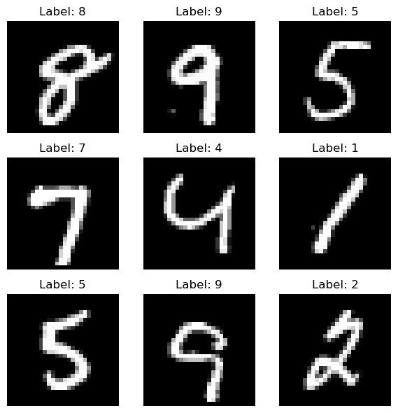
To make this data more intuitive, we randomly select 9 samples, reshape each one into a 28×28 matrix, and display them as images. Here's what that looks like:
import matplotlib.pyplot as plt
sample_imgs = df.sample(9)
fig, axes = plt.subplots(3, 3, figsize=(6, 6))

for i, ax in enumerate(axes.flat):
    img = sample_imgs.iloc[i, :-1].values.reshape(28, 28)
    label = sample_imgs.iloc[i, -1]
    ax.imshow(img, cmap='gray')
    ax.set_title(f"Label: {label}")
    ax.axis('off')

plt.tight_layout()
plt.show()
The code is also pretty simple:
df.sample(9) randomly picks 9 digits from the dataset.
Each image is reshaped from a flat vector back to a 28x28 grid using .reshape(28, 28).
matplotlib is used to plot the images in a 3×3 grid.
The labels are shown above each image so you know what digit it represents.
This simple visualization makes the data feel real as it's no longer just numbers in a table. We're now looking at actual handwriting that our model will soon learn to recognize.
Interestingly, if you look closely at the pixel matrix (without formatting or reshaping), you can actually make out the shape of a digit just from the raw numbers. This works because non-zero values represent the strokes of the handwritten digit.
Let’s bring that to life by visualizing one digit as a heatmap, where brighter colors indicate higher pixel intensity (i.e. more ink):
import matplotlib.pyplot as plt

# Grab the first sample image (excluding the label) and reshape it
img_matrix = sample_imgs.iloc[0, :-1].values.reshape(28, 28)

plt.imshow(img_matrix, cmap='hot')
plt.title(f"Heatmap of Digit: {sample_imgs.iloc[0, -1]}")
plt.axis('off')
plt.show()
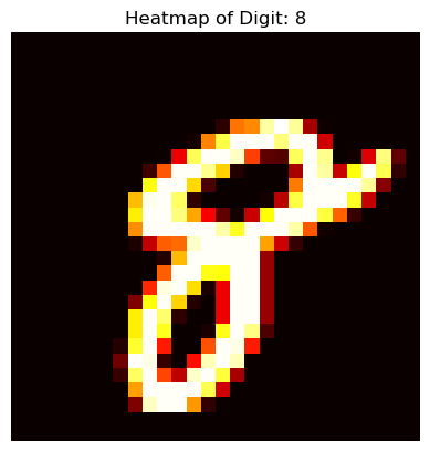
We're using the 'hot' colormap to highlight areas of high intensity.
Bright (yellow/white) regions represent the strokes of the digit.
Darker (black/red) areas are the background or "no ink" zones.
This is exactly the kind of structure a neural network will learn to pick up on, where the ink is, how it's shaped, and what patterns define a 6 versus an 8.
Normalize the Pixel Values
Before feeding the data into a neural network, we need to normalize the pixel values.
Why? Because each pixel is a value between 0 and 255, and neural networks perform better when the input values are on a smaller, consistent scale typically between 0 and 1.
from sklearn.model_selection import train_test_split

# Split features and labels
X = df.iloc[:, :-1].values / 255.0  # normalize
y = df.iloc[:, -1].values

# Train-test split
X_train, X_test, y_train, y_test = train_test_split(X, y, test_size=0.2, random_state=42)
We divide every pixel by 255 to convert values from the range [0, 255] to [0, 1]. This small step improves training speed and stability.
Reshape for CNN Input
Convolutional Neural Networks (CNNs) expect input data with height, width, and channels. Right now, each image is a flat vector of 784 values.
Let’s reshape it into (28, 28, 1) format the last dimension 1 is for grayscale (1 channel).
X_train = X_train.reshape(-1, 28, 28, 1)
X_test = X_test.reshape(-1, 28, 28, 1)
The -1 tells NumPy to automatically figure out the batch size. We’re just reshaping each image from a 1D vector into a 2D matrix with a single channel.
Now that our data is cleaned and reshaped properly, let’s define a Convolutional Neural Network using PyTorch
CNNs are especially good at capturing spatial patterns in images. Instead of treating pixels as independent features (like in a basic neural network), CNNs use filters to scan across images and learn patterns like edges, curves, and ultimately digits.
import torch
import torch.nn as nn
import torch.nn.functional as F
from torch.utils.data import DataLoader, TensorDataset
from sklearn.model_selection import train_test_split
Prepare the Data
We prepare the data by first separating the pixel values (features) from the labels (digit classes), then normalize the features by dividing by 255.0 to scale pixel values to the [0, 1] range, which helps the neural network train more effectively. After splitting the data into training and test sets, we reshape each image into the (1, 28, 28) format expected by PyTorch CNNs, where 1 is the number of color channels (grayscale). We then convert the NumPy arrays into PyTorch tensors, and wrap them in TensorDataset objects. Finally, we use DataLoader to efficiently batch and shuffle the data for training and evaluation.
# Split features and labels
X = df.iloc[:, :-1].values / 255.0
y = df.iloc[:, -1].values

# Train-test split
X_train, X_test, y_train, y_test = train_test_split(X, y, test_size=0.2, random_state=42)

# Reshape and convert to PyTorch tensors
X_train_tensor = torch.tensor(X_train.reshape(-1, 1, 28, 28), dtype=torch.float32)
y_train_tensor = torch.tensor(y_train, dtype=torch.long)
X_test_tensor = torch.tensor(X_test.reshape(-1, 1, 28, 28), dtype=torch.float32)
y_test_tensor = torch.tensor(y_test, dtype=torch.long)

# Create datasets and dataloaders
train_dataset = TensorDataset(X_train_tensor, y_train_tensor)
test_dataset = TensorDataset(X_test_tensor, y_test_tensor)
train_loader = DataLoader(train_dataset, batch_size=64, shuffle=True)
test_loader = DataLoader(test_dataset, batch_size=64)
Define the CNN Model
We define the CNN model to create a neural network architecture that is specifically designed to process image data by learning spatial patterns. Convolutional layers (conv1 and conv2) detect local features like edges and curves, while max pooling layers reduce the spatial dimensions to make the model more efficient and reduce overfitting. The output from the convolutional layers is flattened and passed through fully connected layers (fc1 and fc2) to make predictions. We also use ReLU activations for non-linearity and a dropout layer to help prevent overfitting during training. This architecture transforms input images into class scores representing the digits 0 through 9.
class CNN(nn.Module):
    def __init__(self):
        super(CNN, self).__init__()
        self.conv1 = nn.Conv2d(1, 32, 3, padding=1)
        self.pool = nn.MaxPool2d(2, 2)
        self.conv2 = nn.Conv2d(32, 64, 3, padding=1)
        self.fc1 = nn.Linear(64 * 7 * 7, 64)
        self.dropout = nn.Dropout(0.5)
        self.fc2 = nn.Linear(64, 10)

    def forward(self, x):
        x = self.pool(F.relu(self.conv1(x)))  # 28x28 → 14x14
        x = self.pool(F.relu(self.conv2(x)))  # 14x14 → 7x7
        x = x.view(-1, 64 * 7 * 7)
        x = F.relu(self.fc1(x))
        x = self.dropout(x)
        x = self.fc2(x)
        return x

model = CNN()
Train the Model
We train the model to adjust its internal parameters (weights and biases) so it can accurately classify handwritten digits. This process uses the training data to minimize prediction errors over multiple epochs. We define a loss function (CrossEntropyLoss) that measures how far the model's predictions are from the actual labels, and use the Adam optimizer to update the model’s parameters based on this loss. For each batch of data, we perform a forward pass to get predictions, compute the loss, backpropagate the error, and update the weights. Tracking the running loss and accuracy over each epoch helps us monitor the learning progress.
import torch.optim as optim

criterion = nn.CrossEntropyLoss()
optimizer = optim.Adam(model.parameters(), lr=0.001)

for epoch in range(10):
    running_loss = 0.0
    correct = 0
    total = 0

    for inputs, labels in train_loader:
        optimizer.zero_grad()
        outputs = model(inputs)
        loss = criterion(outputs, labels)
        loss.backward()
        optimizer.step()

        running_loss += loss.item()
        _, predicted = torch.max(outputs, 1)
        total += labels.size(0)
        correct += (predicted == labels).sum().item()

    print(f"Epoch {epoch+1}, Loss: {running_loss:.3f}, Accuracy: {100 * correct / total:.2f}%")
Epoch 1, Loss: 386.764, Accuracy: 85.88%
Epoch 2, Loss: 150.673, Accuracy: 94.69%
Epoch 3, Loss: 116.227, Accuracy: 95.82%
Epoch 4, Loss: 99.392, Accuracy: 96.49%
Epoch 5, Loss: 88.411, Accuracy: 96.71%
Epoch 6, Loss: 79.443, Accuracy: 97.05%
Epoch 7, Loss: 70.979, Accuracy: 97.34%
Epoch 8, Loss: 63.954, Accuracy: 97.54%
Epoch 9, Loss: 60.638, Accuracy: 97.70%
Epoch 10, Loss: 57.378, Accuracy: 97.73%
During training, the model gradually improves its ability to classify handwritten digits by minimizing the loss and increasing accuracy across epochs. In the first epoch, the model starts with a relatively high loss (386.764) and an initial accuracy of 85.88%. As training progresses, the loss consistently decreases while accuracy steadily increases, reaching 97.54% by epoch 8. This shows that the model is learning useful features from the data and becoming more confident in its predictions, with less error and better performance over time.
Evaluate the Model on Test Set
model.eval()  # set to evaluation mode

correct = 0
total = 0

with torch.no_grad():  # disable gradient tracking for inference
    for inputs, labels in test_loader:
        outputs = model(inputs)
        _, predicted = torch.max(outputs.data, 1)
        total += labels.size(0)
        correct += (predicted == labels).sum().item()

print(f"Test Accuracy: {100 * correct / total:.2f}%")
Test Accuracy: 99.04%
import matplotlib.pyplot as plt
# Get a small batch of test images
dataiter = iter(test_loader)
images, labels = next(dataiter)
# Run the model on this batch
outputs = model(images)
_, preds = torch.max(outputs, 1)
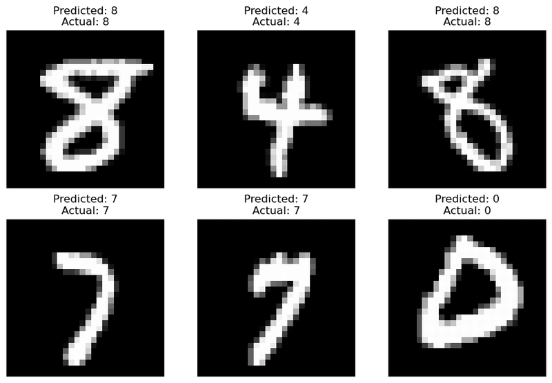
# Plot the first 6 images with predictions
fig, axes = plt.subplots(2, 3, figsize=(9, 6))
for i, ax in enumerate(axes.flat):
img = images[i].squeeze().numpy() # remove channel dimension
ax.imshow(img, cmap='gray')
ax.set_title(f"Predicted: {preds[i].item()}\nActual: {labels[i].item()}")
ax.axis('off')
plt.tight_layout()
plt.show()
Lets show a a visual representation of how the training loss and accuracy evolved over 8 epochs
import matplotlib.pyplot as plt

# Training metrics from the user-provided output
epochs = list(range(1, 9))
loss = [386.764, 150.673, 116.227, 99.392, 88.411, 79.443, 70.979, 63.954]
accuracy = [85.88, 94.69, 95.82, 96.49, 96.71, 97.05, 97.34, 97.54]

# Plotting
fig, ax1 = plt.subplots(figsize=(10, 5))

color = 'tab:red'
ax1.set_xlabel('Epoch')
ax1.set_ylabel('Loss', color=color)
ax1.plot(epochs, loss, marker='o', color=color, label='Loss')
ax1.tick_params(axis='y', labelcolor=color)
ax1.set_title('Training Loss and Accuracy Over Epochs')

# Second y-axis for accuracy
ax2 = ax1.twinx()
color = 'tab:blue'
ax2.set_ylabel('Accuracy (%)', color=color)
ax2.plot(epochs, accuracy, marker='s', linestyle='--', color=color, label='Accuracy')
ax2.tick_params(axis='y', labelcolor=color)

fig.tight_layout()
plt.grid(True)
plt.show()
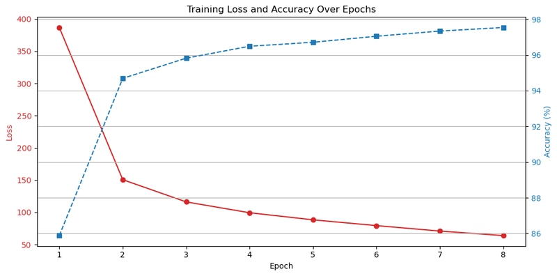
As the loss sharply decreases, the accuracy steadily increases indicating that the model is learning meaningful features from the MNIST dataset.
Conclusion
Through this project, we’ve seen how convolutional neural networks (CNNs) can effectively learn to classify handwritten digits using the MNIST dataset. Starting from data preprocessing and normalization, to reshaping images for CNN input, and finally building and training a deep learning model using PyTorch we’ve followed the complete image classification pipeline. With over 99% accuracy on the test set, the results clearly highlight the power of CNNs in computer vision tasks. As AI continues to evolve, foundational projects like this provide essential insights into how machines learn to see and understand visual data. Whether you're building digit recognizers or training models for more complex vision problems, these techniques remain core building blocks.