


![Apple Developing AI 'Vibe-Coding' Assistant for Xcode With Anthropic [Report]](https://www.iclarified.com/images/news/97200/97200/97200-640.jpg)
![Apple's New Ads Spotlight Apple Watch for Kids [Video]](https://www.iclarified.com/images/news/97197/97197/97197-640.jpg)


_Inge_Johnsson-Alamy.jpg?width=1280&auto=webp&quality=80&disable=upscale#)


![[The AI Show Episode 145]: OpenAI Releases o3 and o4-mini, AI Is Causing “Quiet Layoffs,” Executive Order on Youth AI Education & GPT-4o’s Controversial Update](https://www.marketingaiinstitute.com/hubfs/ep%20145%20cover.png)


![From Art School Drop-out to Microsoft Engineer with Shashi Lo [Podcast #170]](https://cdn.hashnode.com/res/hashnode/image/upload/v1746203291209/439bf16b-c820-4fe8-b69e-94d80533b2df.png?#)


From a Point to L∞
How AI uses distance The post From a Point to L∞ appeared first on Towards Data Science.

Why you should read this
As someone who did a Bachelors in Mathematics I was first introduced to L¹ and L² as a measure of Distance… now it seems to be a measure of error — where have we gone wrong? But jokes aside, there seems to be this misconception that L₁ and L₂ serve the same function — and while that may sometimes be true — each norm shapes its models in drastically different ways.
In this article we’ll travel from plain-old points on a line all the way to L∞, stopping to see why L¹ and L² matter, how they differ, and where the L∞ norm shows up in AI.
Our Agenda:
- When to use L¹ versus L² loss
- How L¹ and L² regularization pull a model toward sparsity or smooth shrinkage
- Why the tiniest algebraic difference blurs GAN images — or leaves them razor-sharp
- How to generalize distance to Lᵖ space and what the L∞ norm represents
A Brief Note on Mathematical Abstraction
You might have have had a conversation (perhaps a confusing one) where the term mathematical abstraction popped up, and you might have left that conversation feeling a little more confused about what mathematicians are really doing. Abstraction refers to extracting underlying patters and properties from a concept to generalize it so it has wider application. This might seem really complicated but take a look at this trivial example:
A point in 1-D is x = x₁; in 2-D: x = (x₁,x₂); in 3-D: x = (x₁, x₂, x₃). Now I don’t know about you but I can’t visualize 42 dimensions, but the same pattern tells me a point in 42 dimensions would be x = (x₁, …, x₄₂).
This might seem trivial but this concept of abstraction is key to get to L∞, where instead of a point we abstract distance. From now on let’s work with x = (x₁, x₂, x₃, …, xₙ), otherwise known by its formal title: x∈ℝⁿ. And any vector is v = x — y = (x₁ — y₁, x₂ — y₂, …, xₙ — yₙ).
The “Normal” Norms: L1 and L2
The key takeaway is simple but powerful: because the L¹ and L² norms behave differently in a few crucial ways, you can combine them in one objective to juggle two competing goals. In regularization, the L¹ and L² terms inside the loss function help strike the best spot on the bias-variance spectrum, yielding a model that is both accurate and generalizable. In Gans, the L¹ pixel loss is paired with adversarial loss so the generator makes images that (i) look realistic and (ii) match the intended output. Tiny distinctions between the two losses explain why Lasso performs feature selection and why swapping L¹ out for L² in a GAN often produces blurry images.

L¹ vs. L² Loss — Similarities and Differences

- If your data may contain many outliers or heavy-tailed noise, you usually reach for L¹.
- If you care most about overall squared error and have reasonably clean data, L² is fine — and easier to optimize because it is smooth.
Because MAE treats each error proportionally, models trained with L¹ sit nearer the median observation, which is exactly why L¹ loss keeps texture detail in GANs, whereas MSE’s quadratic penalty nudges the model toward a mean value that looks smeared.
L¹ Regularization (Lasso)
Optimization and Regularization pull in opposite directions: optimization tries to fit the training set perfectly, while regularization deliberately sacrifices a little training accuracy to gain generalization. Adding an L¹ penalty